Distribution Model Tool
With the Distribution Model Tool, you can create probability distribution models to display on histograms and/or to assign them on the Transform and Trends form in the Rock Property modeling workflow. To open the tool, click the edit  icon, next to the 'Name' drop-down on the Distribution Model tab on the Histogram Tool.
At the top of the Distribution Model Tool, you can use the toolbar to duplicate, rename, or delete your existing distribution models.

|
Duplicates the currently selected item in the drop-down list (i.e., the active item). |

|
Opens the Rename dialog, where a new name can be given to the active item. |

|
Deletes the active item. |
To create a distribution model
- Select
 Create new from the Distribution model drop-down list. Optionally, enter the name of the distribution model in text field below. By default, a new distribution model is named as 'Distribution Model <#>'. To modify the name of an existing distribution model, use the rename button
  .
. - The following fields are populated as read-only:
- Source chart The name of the histogram (selected in the Histogram Tool). This source chart is used when you select the Autofit to Data option below. If you close the Histogram Tool while working on the Distribution Model Tool, this entry is grayed out and the Autofit to Data option is disabled.
- Source series The name of the series for which you are creating the distribution model. This source series is used to make sure that the property types of the histogram and distribution model match. If you close the Histogram Tool while working on the Distribution Model Tool, this entry is grayed out and the Autofit to Data option is disabled.
- Property type The property type or log type of the source series (from the Data tab in the Histogram Tool). If you close the Histogram Tool while working on the Distribution Model Tool, you can select a property type.
- From the Type drop-down list, select one of the following distribution model types: Gaussian, Lognormal, Triangular, or Uniform. The tool displays the corresponding model parameters.
- Click the Autofit to Data
 button (recommended) to fill in the distribution model parameters. The autofit is based on the data belonging to the source chart and series selected at the top of the form. You can also manually enter the parameter values.
 - Click Apply to create the distribution model and keep the tool open or click OK to create the distribution model and close the tool. The distribution model is immediately selected on the Histogram Tool.
- Return to the Distribution Model tab on the on the Histogram Tool. To visualize the distribution model on the histogram, click Apply and keep the tool open, or click OK and close the tool.
You can view and adjust these parameters for the distribution models:
Type Select the distribution type from the drop-down list. You can select from one of the following models: Gaussian, Lognormal, Triangular, or Uniform.
Minimum/Maximum (Only for uniform and triangular distributions) Enter the minimum and maximum values for the distribution model.
Mode (Only for triangular distribution) Enter the mode (most likely) value of the distribution model.
Mean (Only for Gaussian and lognormal distribution) Enter the average of the distribution model. The mean of a lognormal model must be positive.
Standard deviation (Only for Gaussian and lognormal distribution) Enter the standard deviation of the distribution model. This is the measure of how dispersed the data is in relation to the mean. The standard deviation must be positive.
Truncation settings remove the tails of Gaussian, lognormal, and (optionally) triangular distribution models.
Apply truncation (Optional for triangular distribution) Check the checkbox to enable the minimum and maximum truncation fields.
Minimum/Maximum truncation (Mandatory for Gaussian and lognormal distribution) These settings control the limits of truncated distribution models. Enter the minimum and maximum values for the truncation. For a lognormal model these must both be positive.
Weighting
The Unweighted and Weighted options control whether 'Autofit to Data' is performed without or with data weights. The Weighted option is only available for data from a 3D grid, where the cell volumes are used as weights, and well-log data, where the sample spacings are used as weights.
How to use the 'Autofit to Data' button
Click the Autofit to Data button ![]() to automatically populate the model parameters (using the data from the Source chart and Source series) and calibrate them using the 'method of moments'. Statistics of the model are matched to the corresponding statistics of the data. The table below shows the calculations performed and which model parameter fields are populated.
to automatically populate the model parameters (using the data from the Source chart and Source series) and calibrate them using the 'method of moments'. Statistics of the model are matched to the corresponding statistics of the data. The table below shows the calculations performed and which model parameter fields are populated.
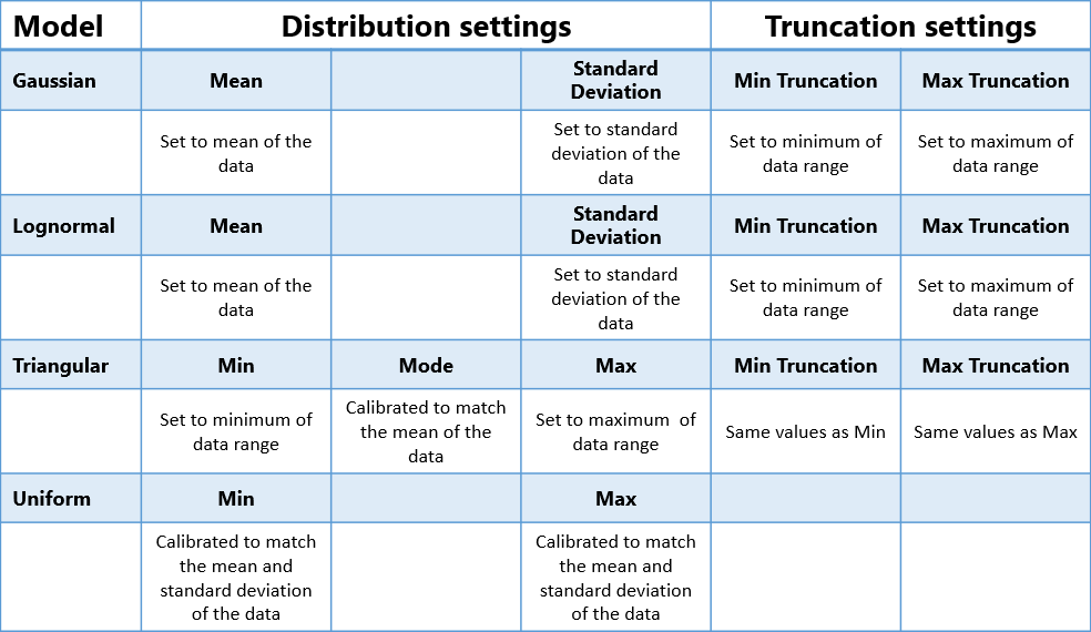
The calculations performed and fields populated by the Autofit to data button. Note that the data for Uniform models might extend beyond the range of the model. click to enlarge